Tutorial
This guide will help you start working with PyRayT by designing and simulating a collimating lens.
Creating Components
We’re going to create a biconvex lens (one of the many built in lens types) with a radius of curvature of 2 “world units”. PyRayT does not enforce a specific unit system so 2 can be meters, feet, inches, or angstroms! Since most optical components are specified in inches, however, we’ll imagine it’s a lens with a 2” radius of curvature, and a 1” aperture. This is a thick lens so we also need to specify a thickness, for now we’ll use 0.25”.
import pyrayt
lens = pyrayt.components.biconvex_lens(r1=2, r2=2, thickness=0.25, aperture=1)
We can look at the lens using the TinyGfx draw() function.
from tinygfx.g3d.renderers import draw
draw(lens)
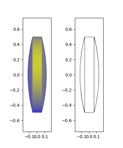
The default options for draw will shade the lens with a Gooch Shader. For an edge renderer, use the optional shaded=False
argument.
Moving an Object in 3D Space
On creation, the lens is centered at the world origin with the optical axis colinear to the x-axis. All optical components can be
moved around in world space using WorldObject methods. These methods update the component’s relative
position in space, and can be chained together in one line. For example, below are separate ways to move the lens to (3,2,1)
# chaining multiple move_axis calls
lens.move_x(3).move_y(2).move_z(1)

# using the move method for all three axes at once
lens.move(3,2,1)

# using one movement call per line
lens.move_x(3)
lens.move_y(2)
lens.move_z(1)

# Successive calls to the same movement method
lens.move_x(5)
lens.move_x(-2).move_y(2).move_z(1)
The position of the lens can be checked with get_position(). The returned
value is a 4D HomogeneousCoordinate, with dimensions of [x, y, z, w]
lens.get_position()
Point([0., 0., 0., 1.])
lens.get_position.x
0.0
Rotation
In addition to movement, components can be rotated about the principle axes, not the body center. The orientation of an optical component can be checked with get_orientation() which returns a vector pointing along the components axis. By default our lens is pointing towards the positive X axis.
lens.get_orientation()
Vector([ 1.0, 0.0, 0.0 , 0.0])
lens.get_position()
Point([0., 0., 0., 1.])
lens.rotate_z(90).move_x(5)
lens.get_orientation()
Vector([ 0.0, 1.0, 0.0 , 0,0])
lens.get_position()
Point([5., 0., 0., 1.])
Unlike movement, the order that operations are chained does matter for rotations. As a reference, if you want to rotate a component, apply rotations while it is centered at the world origin and then move.
Operation |
Final Position |
Final Orientation |
|---|---|---|
|
(0, 5, 0) |
(0, 1, 0) |
|
(5, 0, 0) |
(0, 1, 0) |
Adding Sources
A ray tracer wouldn’t be very interesting if it didn’t have a way to generate rays! In PyRayT this is handled by various sources. The one we’ll be working with is pyrayt.components.ConeOfRays, which generates a uniformly distributed set of rays that all make the same angle to the optical axis.
source = pyrayt.components.ConeOfRays(cone_angle=10)
Notice that when creating the source, we don’t specify how many rays it should generate, that’s because ray generation is handled by a RayTracer object. This allows for the same ray trace to be used for quick visual simulations with a small number of rays, as well as for larger simulations with 100k+ rays, without ever having to redefine the system.
Like our lens, sources can be moved in world space. We’re going to keep the lens at the origin, but move the source along the -x axis until it is at the lens’ focal point, this will cause any rays from our source to be collimated when they hit the lens. The focal length of the lens is 2.04” from the lensmaker’s equation (by default lenses have a refractive index of 1.5 across all wavelengths, set by the lens’ material).
f = 2.04
source.move_x(-f)
Performing a Ray Trace
In a world where we don’t trust the lensmaker’s equation, we’d want to verify that rays originating at a lens’ derived focal point are actually collimated. To do this we’ll perform a ray trace with the RayTracer object.
When creating a ray tracer, you need to provide all sources and components that will be part of the traced system. Since we only have one source and one component, it’s pretty simple. We’re also going to set how many rays the trace will generate for each source, as well as the generation limit for the rays. generation_limit is a parameter of the ray trace that specifies how many ray-surface interactions a unique ray can have before it is terminated by the ray tracer.
tracer = pyrayt.RayTracer(sources=source, components=lens)
tracer.set_rays_per_source(10)
tracer.set_generation_limit(100)
The ray tracer only receives a reference to our source and lens, not copies of them. Due to this, you can continue to move components around after creating a RayTrace object, and the updated positions will be used when a trace is performed.
The ray trace is run with the trace() method, which returns a Pandas dataframe of the simulation results.
results = tracer.trace()
Analyzing Results
Before diving into the raw data, we want to take a look at the resulting trace to make sure it matches what we expect. This is accomplished with the show() method.
tracer.show()
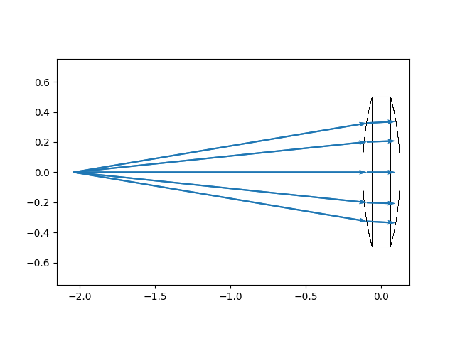
It’s a good thing we checked because this is not what we want to see! The rays generate fine and interact with the lens, but instead of leaving the lens they terminate at the back surface. This means we have no way to know if the lens actually collimates the rays or not. From the ray tracer’s perspective, however, it accomplished its job without error.
At every generation the ray tracer checks if the ray intersects any surface in the simulation. If it can’t find an intersection, the ray tracer considers that ray as no longer part of our simulation and terminates it. In order to verify the rays are collimated, we need to add a second surface after the lens that the rays can interact with. For that we’ll add a baffle().
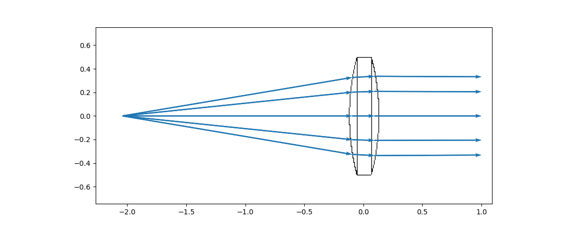
Baffles are generic components that mimic a perfect absorber, any ray that intersects a baffle is terminated and removed from the simulation. However, since the baffle is part of the simulation components, those rays will be stored in the ray trace as terminating on that surface instead of being eliminated unceremoniously. This makes it perfect for modelling things like imagers, photodiodes, or apertures. let’s add a baffle to the ray trace and move it along the positive x-axis some distance away from the lens.
baffle = pyrayt.components.baffle((1,1))
tracer.load_system([lens, baffle])
baffle.move_x(1)
Now when we run the ray trace we get the results we’d expect. Unfortuately you still cannot see the baffle, even though the rays interact with it. This is because the draw() function itself is performing a ray trace, where each pixel value is the result of a ray projected into the scene! Since the baffle has no depth and is perpendicular to the viewing plane, it’s impossible for a ray to intersect with it.
Note
3D rendering of components for ray trace results is an area that is actively being worked on. Contributions are welcome from anybody with 3D/OpenGL experience.
Processing Ray Data
A picture might be worth 1000 words, but sometimes we need to dig into the numerical data of a ray trace itself. This is where the results dataframe comes in. The dataframe details are covered in the Reference section, but we’ll quickly cover how to use it to extract quantitative data about the simulation.
first, lets dump the result to the repl and see how the data is stored
results
    generation  intensity  wavelength  ...    x_tilt        y_tilt    z_tilt
0          0.0      100.0       0.633  ...  0.984808  0.000000e+00  0.173648
1          0.0      100.0       0.633  ...  0.984808  1.020678e-01  0.140484
2          0.0      100.0       0.633  ...  0.984808  1.651492e-01  0.053660
3          0.0      100.0       0.633  ...  0.984808  1.651492e-01 -0.053660
4          0.0      100.0       0.633  ...  0.984808  1.020678e-01 -0.140484
5          0.0      100.0       0.633  ...  0.984808  2.126577e-17 -0.173648
6          0.0      100.0       0.633  ...  0.984808 -1.020678e-01 -0.140484
7          0.0      100.0       0.633  ...  0.984808 -1.651492e-01 -0.053660
8          0.0      100.0       0.633  ...  0.984808 -1.651492e-01  0.053660
9          0.0      100.0       0.633  ...  0.984808 -1.020678e-01  0.140484
10         1.0      100.0       0.633  ...  0.998415 -1.992050e-17  0.056272
11         1.0      100.0       0.633  ...  0.998415  3.307579e-02  0.045525
12         1.0      100.0       0.633  ...  0.998415  5.351775e-02  0.017389
13         1.0      100.0       0.633  ...  0.998415  5.351775e-02 -0.017389
14         1.0      100.0       0.633  ...  0.998415  3.307579e-02 -0.045525
15         1.0      100.0       0.633  ...  0.998415 -1.302918e-17 -0.056272
16         1.0      100.0       0.633  ...  0.998415 -3.307579e-02 -0.045525
17         1.0      100.0       0.633  ...  0.998415 -5.351775e-02 -0.017389
18         1.0      100.0       0.633  ...  0.998415 -5.351775e-02  0.017389
19         1.0      100.0       0.633  ...  0.998415 -3.307579e-02  0.045525
20         2.0      100.0       0.633  ...  0.999988  9.597537e-20 -0.004965
21         2.0      100.0       0.633  ...  0.999988 -2.918377e-03 -0.004017
22         2.0      100.0       0.633  ...  0.999988 -4.722033e-03 -0.001534
23         2.0      100.0       0.633  ...  0.999988 -4.722033e-03  0.001534
24         2.0      100.0       0.633  ...  0.999988 -2.918377e-03  0.004017
25         2.0      100.0       0.633  ...  0.999988 -5.120666e-19  0.004965
26         2.0      100.0       0.633  ...  0.999988  2.918377e-03  0.004017
27         2.0      100.0       0.633  ...  0.999988  4.722033e-03  0.001534
28         2.0      100.0       0.633  ...  0.999988  4.722033e-03 -0.001534
29         2.0      100.0       0.633  ...  0.999988  2.918377e-03 -0.004017
[30 rows x 15 columns]
Our results dataframe has 30 rows and 15 columns. Every row is a unique ray segment and each column represents a piece of metadata for that segment. According to the ray trace settings though, we only generated 10 rays for our source. So why are there 30 different rays saved? This is because a ray’s metadata is only valid until it intersects another surface. Imagine this: we have a ray in air that refracts into water. The refractive index, tilt, and intensity all need to be updated because of this refraction, but we don’t want to lose track of what those values were when the ray was originally in air.
To handle this, PyRayT splits rays into segments where the metadata is valid for that entire segment. When a ray intersects a surface, a new segment is made with the generation number of the ray incremented by 1.
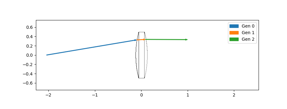
All rays have a unique id that is stored with each segment, so it is still possible to trace a single ray’s path through a system. For example, lets take a look at all the segments for the ray with id=0.
results.loc[results['id']==0]
    generation  intensity  wavelength  ...    x_tilt        y_tilt    z_tilt
0          0.0      100.0       0.633  ...  0.984808  0.000000e+00  0.173648
10         1.0      100.0       0.633  ...  0.998415 -1.992050e-17  0.056272
20         2.0      100.0       0.633  ...  0.999988  9.597537e-20 -0.004965
[3 rows x 15 columns]
This ray is composed of three segments. Plotting the trace again for just this ray we can see that new segments are generated when we enter and exit the lens. Since the baffle absorbs the ray, no new segments are generated after that intersection.
Taking it Further
This demonstration showed only a few of the features PyRayT has to offer. Take a look in the Reference for more information on each part of the ray tracer flow, or check out Additional Examples for designs to try out.